Development of a 2D+ dynamic model of an aluminum reduction cell
Marc Dupuis GéniSim 3111 Alger St., Jonquière, Québec, Canada G7S 2M9 email:
R. Lacroix
Chemical Engineering Dept.
Laval University
Ste-Foy, Québec, Canada G1K 7P4
ABSTRACT
A program was developed to model the dynamic behavior of an aluminum reduction cell. The program simulates the electrolysis process by solving heat and mass balance equations, incorporating the impact of operator events like metal taping and anode changes and reproducing the work of the cell controller.
In this paper, a new finite elements based 2D+ thermal model of the cell is introduced to solve the heat balance equation more rigorously. The dynamic thermal response of the cell using this new more sophisticated thermal model is compared with the more simpler and faster 1D version. Execution time is also compared.
INTRODUCTION
The design and operation of an aluminum reduction cell is a complex task requiring a detailed understanding of the behavior of the cell. To develop a better understanding, it is useful to simulate the cell behavior by using mathematical models.
It is now common practice to develop three types of mathematical models of the cell:
Up to now, it was also common practice to develop two types of thermal-electric models:
Clearly, the complexity of the many interrelated physical and chemical phenomena involved in an aluminum reduction cell still prevents us from building a practical "multi-physics" unified model, the main practical issue being the excessive amount of computer resources required (1).
Yet, for the very reason that they are interrelated, we must remember that the current common practice is the result of a compromise between model accuracy and model manageability. As computer technology continues to evolve, we must keep in mind that the "multi-physics" unified model should be the ultimate goal (2).
The present work represents one step in that direction with the development of a thermal-electric 2D+ dynamic model of an aluminium reduction cell.
ANSYS« 2D+ STEADY STATE MODEL
In a previous publication (3), the state of the art of computing the steady state energy balance of an aluminum reduction cell using ANSYS« finite element models was reviewed. Many 3D models were presented: 3D half anode, 3D cathode side slice, 3D cell side slice, 3D anode panel, 3D cathode quarter and 3D cell quarter. From the above, the 3D cell side slice model can be considered as the current "standard" model.
It has replaced "classic" 2D models (4,5) that are not able to accurately represent the impact of anode studs and cathode collector bar that are discontinuous in the third dimensions. The cost to pay to get that accuracy is the extra CPU time required to solve a 3D cell slice model instead of a "classic" 2D model. Yet, with today computer speed, it is not a big issue anymore as the typical elapsed time to solve such a 3D model is around 30 minutes on a Pentium II 266 MHz processor.
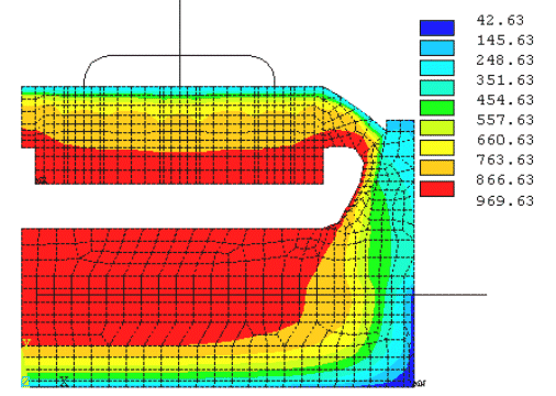
Nevertheless, it was demonstrated (3) that an improved version of the 2D model, called the 2D+ model, could be used to produce results as accurate as the 3D model but 6 times faster. The key to the gained accuracy for the 2D+ model over the "classic" 2D model is the addition of 1D beam elements to represent the third dimension effect of anode studs and cathode collector bars over the "standard" 2D lining mesh (see figure 1).

Figure 1 - Isotherms solution of a 2D+ steady state thermal-electric model
DYNA/MARC 1D DYNAMIC MODEL
Having to wait 30 minutes (or even 5 minutes) to get the solution of one time step in a dynamic simulation that requires thousands of time steps is clearly not a practical option. For that reason, a much simpler 1D model representation have been developed (6). The concept of the simplified 1D thermal model is to assume that the heat produced in the liquid zone of the cell can only travel out of the cell by one of four parallel pathways described in figure 2.
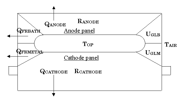
Figure 2 - Schematic of the 1D thermal model concept
Following that concept, the complex heat loss dissipation through the cell lining is simplified to the following six basic equations:
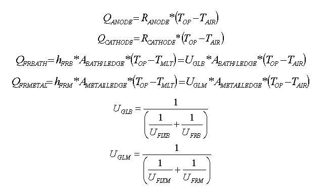
That 1D thermal model has been implemented into a comprehensive dynamic cell model and the temperature evolution predictions have been successfully compared against measurement (7). Because the 1D thermal model is so simple, it takes less that one second to compute the 2160 time steps required to run 3 days of simulation using a time step size of 2 minutes (see figure 3).
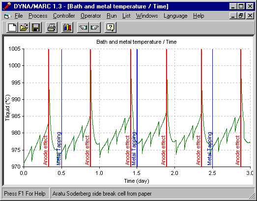
Figure 3 - Temperature evolution using DYNA/MARC 1D dynamic model
ANSYS« 2D+ DYNAMIC MODEL
As presented in previous publications (8-9), the 1D thermal model is a very powerful tool to quickly analyze "what if" scenario and run Monte Carlo risk assessment analysis because it provides fast and fairly accurate steady state solution.
Yet, because its formulation does not account for the thermal mass latent heat effect of the cell cathode lining and anode cover, the prediction of the 1D thermal model cannot be accurate in rare occasions like long anode effects or long power loss events where this effect becomes important.
In order to be able to accurately predict the thermal response of those exceptional events, an ANSYS« 2D+ dynamic model has been developed. The model is a mix of the ANSYS« 2D+ model that is run in transient mode and an extensive APDL macro that computes the heat and mass balances of the liquid zone of the cell in a way similar to what DYNA/MARC does (10). The only difference between the DYNA/MARC model and the APDL macro of the 2D+ dynamic model is that the 1D thermal submodel in DYNA/MARC has been replaced by the ANSYS« 2D+ thermal-electric submodel.
MODELS RESULTS COMPARISON
Two cases are presented in order to be able to compare the predicted thermal response of both dynamic models. In the first case, the usual one-hour thermal response of a standard PBF underfeeding-overfeeding cycle is presented. In the second case, the unusual one-hour thermal response of a total line power failure is presented.
Normal operation
Starting from the steady state solution, both simulations begin at 75% of the nominal underfeeding regime and will carry on that feeding regime until the cell resistance slope reaches 0.003 m-ohm/min. At that time, the feeding regime is shifted to 140% of nominal overfeeding for 30 minutes. No other events are affecting the operation of the cell in those simulations. In both cases, the time step size was set to 2 minutes.
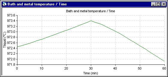
Figure 4 - Temperature evolution using DYNA/MARC 1D dynamic model
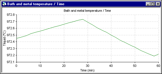
Figure 5 - Temperature evolution using ANSYS« 2D+ dynamic model
Apart from the shift to the overfeeding that occurs after 28 minutes in the 2D+ run instead of 30 minutes for the 1D run, the trend of the temperature evolution is the same. Yet, the amplitude of the fluctuation is reduced significantly in the 2D+ run. Following are the cell superheat evolution results. Note that in both simulations, the eutectic superheat was selected to evaluate the heat transfer at the ledge interface.
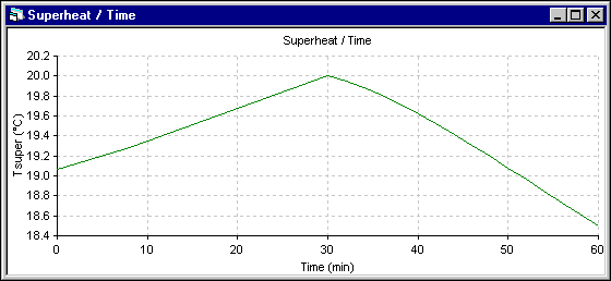
Figure 6 - Eutectic superheat evolution using DYNA/MARC 1D dynamic model
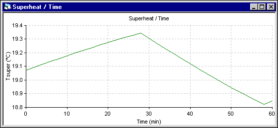
Figure 7 - Eutectic superheat evolution using ANSYS« 2D+ dynamic model
The superheat evolution follows very closely the temperature evolution, so the superheat increases more in the 1D model. The next results presented are those of the energy required to melt (+) or make (-) ledge which is directly proportional to the ledge melting rate. Following the assumptions of the 1D model, the melting rate is primarily function of the superheat. For the 2D+ model, at the end of each time step, the ledge motion macro is used to maintain the ledge surface at the current eutectic temperature. The melting rate is obtained by computing the ledge thickness change between two time steps.
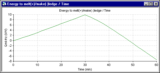
Figure 8 - Energy to melt ledge (+) evolution using DYNA/MARC 1D dynamic model
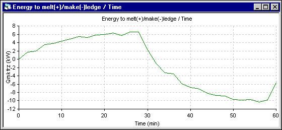
Figure 9 - Energy to melt ledge (+) evolution using ANSYS« 2D+ dynamic model
Finally, the last results presented are the average ledge thickness evolution at the bath level. Obviously, for the 1D model, the average thickness is the only value computed. For the 2D+ model, the average thickness is computed from the ledge profile evolution. For the 1D model, the ledge thickness stops to melt when the cell superheat reaches back to its initial steady state value. For the 2D+ model, the ledge thickness evolution follows more directly the superheat evolution.
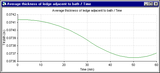
Figure 10 - Bath ledge thickness evolution using DYNA/MARC 1D dynamic model
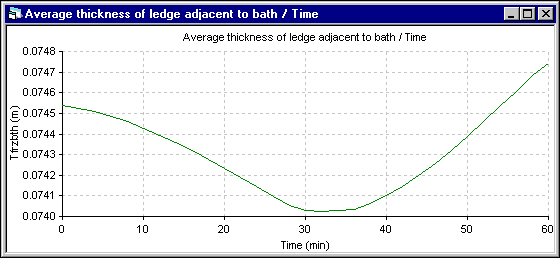
Figure 11 - Bath ledge thickness evolution using ANSYS« 2D+ dynamic model
Considering that the solution of the DYNA/MARC 1D dynamic model was obtained in a fraction of second while the ANSYS« 2D+ dynamic model took 2629.7 seconds CPU or 1 hour and 26 minutes of elapsed time to compute the solution, the 1D model results can be considered as quite acceptable.
The above example demonstrates that neglecting the thermal mass effect of the cell lining generates an offset of less than one degree on the temperature response. Obviously, this kind of difference cannot be measured experimentally.
Power loss
Yet there is rare and extreme events where the thermal mass of the cell lining will have a measurable impact on the temperature evolution. One such event is a total power loss on the line.
In this second case, starting from the same steady state initial conditions, both dynamic simulation are carried out at 1 kA of line current instead of the usual 300 kA. The nominal feeding rate is adjusted accordingly, so the alumina feeding is almost stopped.
In the following two figures, the temperature evolution of both simulation are presented. In the 1D model, the temperature drops very rapidly. But in the 2D+ model, the temperature drops much more slowly as the thermal mass that needs to be cool down is much bigger.
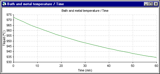
Figure 12: Temperature evolution using DYNA/MARC 1D dynamic model
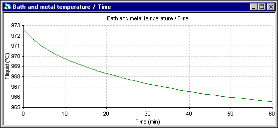
Figure 13: Temperature evolution using ANSYS« 2D+ dynamic model
The energy to make (-) ledge, which is proportional to the ledge thickness evolution rate, is presented next. In the 1D model, this rate is calculated using the Stefan law. So it is set proportionally to the amount of heat getting in (proportional to the superheat) minus the amount of heat going out (inversely proportional to the ledge thickness). In the 2D+ model, the Stefan problem is automatically taking care of by the ledge thickness adjustment in order to keep the ledge surface at the eutectic temperature.
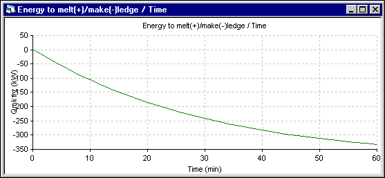
Figure 14: Energy to make ledge (-) evolution using DYNA/MARC 1D dynamic model
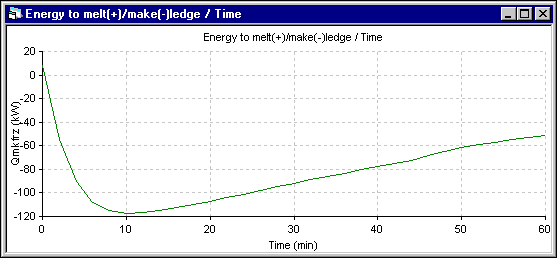
Figure 15: Energy to make ledge (-) evolution using ANSYS« 2D+ dynamic model
The minimum observed in the energy to make ledge (-) in the 2D+ simulation (the maximum ledge growing rate) corresponds to the inflection in the ledge thickness evolution rate presented in the figure 17. This corresponds in the 2D+ simulation to the time where the liquid zone starts to receive heat from the lining instead of giving heat to it. Of course, this effect is not present in the 1D model.
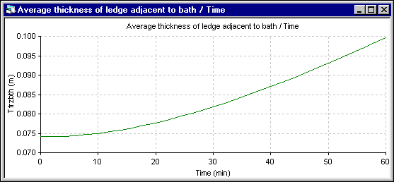
Figure 16: Bath ledge thickness evolution using DYNA/MARC 1D dynamic model
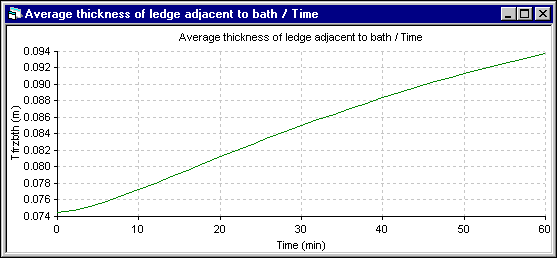
Figure 17: Bath ledge thickness evolution using ANSYS« 2D+ dynamic model
Despite its obvious weakness to predict the correct temperature evolution for that extreme event, the 1D model manages to predict the ledge thickness evolution relatively well considering the fact that the solution was obtained in a fraction of second instead of the 2711.7 seconds CPU or 1 hour 30 minutes of elapsed time required by the 2D+ model.
CONCLUSIONS
An ANSYS« 2D+ dynamic model has been successfully developed and tested. For the 2D+ mesh and the time step selected, the 2D+ model required an hour and a half of elapsed time to simulate an hour of cell operation.
The comparison between the very simple and very efficient 1D model implemented in DYNA/MARC demonstrates that in normal operation, the thermal mass effect of the cell lining is very small.
In retrospect, the success of the simple 1D model to reproduce the thermal evolution of the cell temperature in the Aratu cell (7) can be attributed to the fact that the three main effects that drive the cell temperature evolution in that case are:
and all those effects are well simulated in the DYNA/MARC 1D dynamic model.
The ANSYS« 2D+ dynamic model demonstrated its value to simulate rare extreme events like a long total power loss event where the thermal mass effect of the cell lining cannot be neglected.
REFERENCES